Authors:
(1) Guillaume Staerman, INRIA, CEA, Univ. Paris-Saclay, France;
(2) Marta Campi, CERIAH, Institut de l’Audition, Institut Pasteur, France;
(3) Gareth W. Peters, Department of Statistics & Applied Probability, University of California Santa Barbara, USA.
Table of Links
2.1. Functional Isolation Forest
3. Signature Isolation Forest Method
4.1. Parameters Sensitivity Analysis
4.2. Advantages of (K-)SIF over FIF
4.3. Real-data Anomaly Detection Benchmark
5. Discussion & Conclusion, Impact Statements, and References
Appendix
A. Additional Information About the Signature
C. Additional Numerical Experiments
4.1. Parameters Sensitivity Analysis
We investigate the behavior of K-SIF and SIF with respect to their two main parameters: the depth of the signature k and the number of split windows ω. For the sake of place, the experiment on the depth is postponed in Section C.1 in the Appendix.
The Role of the Signature Split Window. The number of split windows allows the extraction of information over specific intervals (randomly selected) of the underlying data. Thus, at each tree node, the focus will be on a particular portion of the data, which is the same across all the sample curves for comparison purposes. This approach ensures that the analysis is performed on comparable sections of the data, providing a systematic way to examine and compare different intervals or features across the sample curves.
We explore the role of this parameter with two different datasets that reproduce two types of anomaly scenarios. The first considers isolated anomalies in a small interval, while the second contains persistent ones across all the function parametrization. In this way, we observe the behavior of K-SIF and SIF with respect to different types of anomalies.
The first dataset is constructed as follows. We simulate 100 constant functions. We then select at random 90% of these curves and Gaussian noise on a sub-interval; for the remaining 10% of the curves, we add Gaussian noise on another sub-interval, different from the first one. More precisely:
• 90% of the curves, considered as normal, are generated according to

with ε(t) ∼ N (0, 1), b ∼ U([0, 100]) and U representing the uniform distribution.
• 10% of the curves, considered as abnormal, are generated according to

where ε(t) ∼ N (0, 1) and b ∼ U([0, 100]).

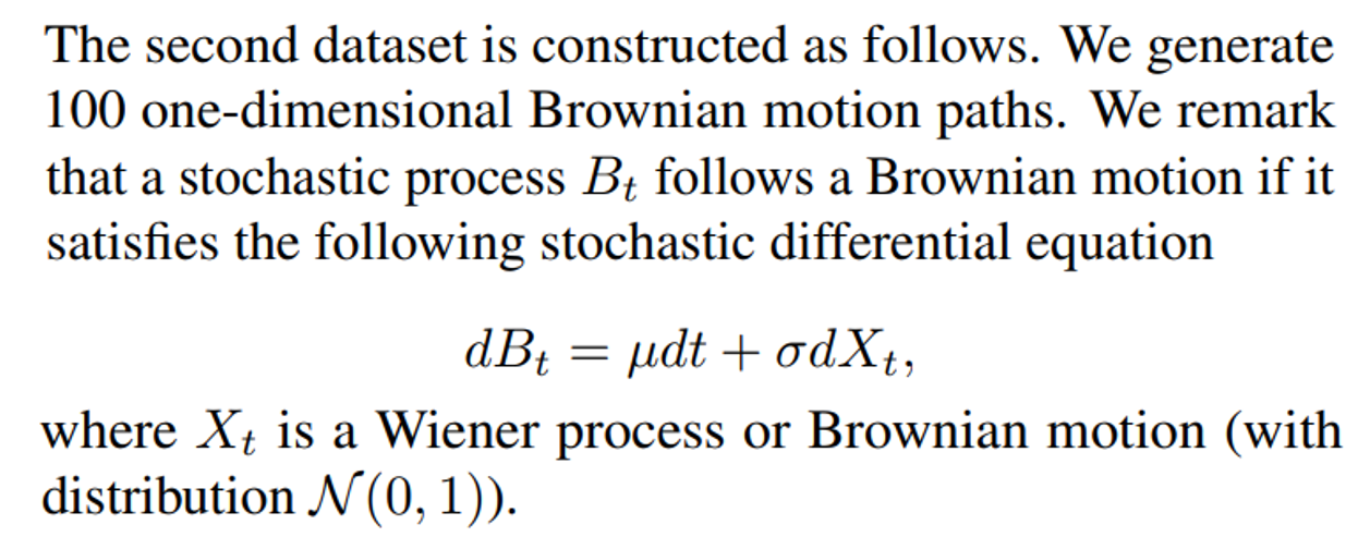
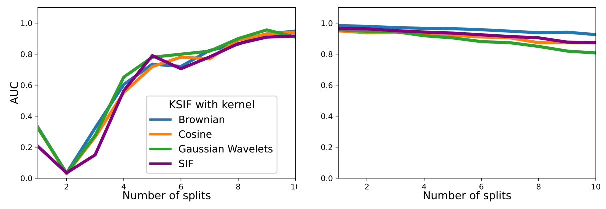
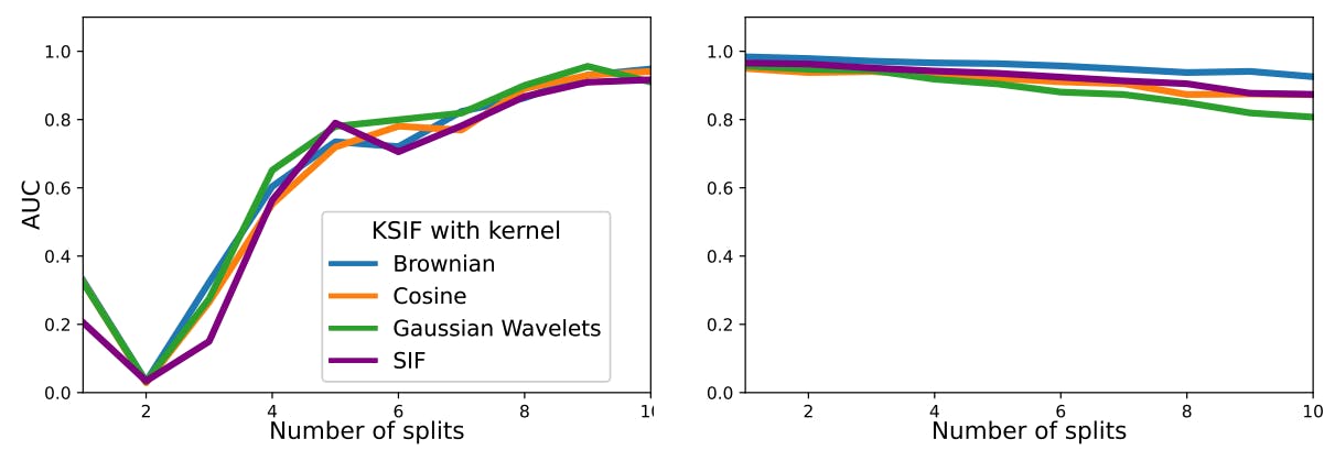
We simulate at random 90% of the paths with µ = 0, σ = 0.5, and consider them as normal data. Then, the remaining 10% are simulated with drift µ = 0.2, standard deviation σ = 0.4, and considered abnormal data. We compute K-SIF with different numbers of split windows, varying from 1 to 10, with a truncation level set equal to 2 and N = 1, 000 the number of trees. The experiment is repeated 100 times, and we report the averaged AUC under the ROC curves in Figure 1 for both datasets and three pre-selected dictionaries.
For the first dataset, where anomalies manifest in a small portion of the functions, increasing the number of splits significantly enhances the algorithm’s performance in detecting anomalies. The performance improvement shows a plateau after nine split windows. In the case of the second dataset with persistent anomalies, a higher number of split windows has a marginal impact on the algorithm’s performance, maintaining satisfactory results. Therefore, without prior knowledge about the data, opting for a relatively high number of split windows, such as 10, would ensure robust performance in both scenarios. Additionally, a more significant number of split windows enables the computation of the signature on a smaller portion of the functions, leading to improved computational efficiency.

This paper is available on arxiv under CC BY 4.0 DEED license.

